Basic usage

Installation

C++

The installation of the C++ version of Open3D is described under Open3D - C++.

It is required to build it from source.

Python

Open3D can be installed from master branch with :

• PIP :

python -c "import open3d as o3d"``pip install --user --pre https://storage.googleapis.com/open3d-releases-master/python-wheels/open3d-0.11.1-cp38-cp38-linux_x86_64.whl

• CONDA :

conda install -c open3d-admin open3d

To quickly test if Open3D is correctly installed, run :

python -c "import open3d as o3d"

You should get a result like <module 'open3d' from 'D:\\Anaconda\\lib\\site-packages\\open3d\\__init__.py'>.

Usage (Python)

A lot of tutorials are presented in the official documentation.

However, the following snippet has been made to have a complete pipeline as in the PCL Toolkit - Pipeline idea for a quick beginning with Open3D.

It is presented step by step, coded like in a Jupyter Notebook.

First block is used to include necessary imports :

#Ensure o3d is running
import open3d as o3d # conda install -c open3d-admin open3d
import numpy as np
import time
from tkinter import Tk #Filepicker
from tkinter.filedialog import askopenfilename
Tk().withdraw()
import copy
import matplotlib.pyplot as plt
print(o3d)

Next, we load a file thanks to a file picker. It has a tendency to appear under already opened windows, so watch for it in your application tab.

It uses the method o3d.io.read_point_cloud(filename) to load a cloud into pcd variable :

#Load pcd file
print("Load PCD file")
filename = askopenfilename()
start_time = time.time()
pcd = o3d.io.read_point_cloud(filename)
elapsed_time = time.time() - start_time
print("Load done in", elapsed_time*1000, "[ms] with", len(pcd.points), "points")

To further apply algorithms, it is often needed to downsample the cloud to have fast running algorithms.

Here, the method is a voxel downsampling, as presented in PCL Toolkit - Downsampling, from previous pcd file pcd.voxel_down_sample(voxel_size=voxelsize) :

#Downsample it
voxelsize = 0.8
print("Downsample the point cloud with a voxel of",voxelsize)
start_time = time.time()
downpcd = pcd.voxel_down_sample(voxel_size=voxelsize)
elapsed_time = time.time() - start_time
print("Downsample done in", elapsed_time*1000, "[ms] from",len(pcd.points),"to",len(downpcd.points),"points")

To trial the alignment process, a second cloud - moved in space - is created.

Here, we translate it thanks to moved_down_pcd.translate((xoff,yoff,zoff)) :

#Creates a moved cloud
xoff = 33
yoff = 36
zoff = 24
moved_down_pcd = copy.deepcopy(downpcd)
print("Move cloud with xoff =",xoff,"yoff =",yoff,"zoff =",zoff)
start_time = time.time()
moved_down_pcd.translate((xoff,yoff,zoff))
elapsed_time = time.time() - start_time
print("Moved cloud done in", elapsed_time*1000)

We can show both clouds in space with :

#Show
print("Show cloud - press H to display commands here")
o3d.visualization.draw_geometries([downpcd,moved_down_pcd])

Giving the following result :

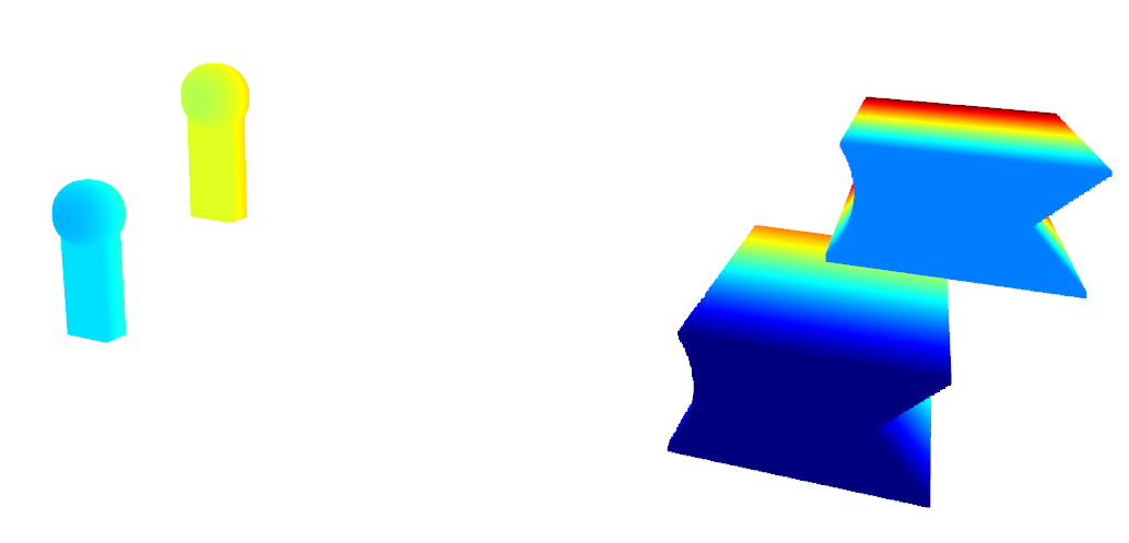
Visualization of the two clouds

Then, we need to calculate the normals to be able to compute FPFH features :

#Calculate features for global registration
        # Add normals
radius_normal = voxelsize * 2
print("Estimate normals of base cloud with radius of",radius_normal)
start_time = time.time()
downpcd.estimate_normals(o3d.geometry.KDTreeSearchParamHybrid(radius=radius_normal, max_nn=30))
elapsed_time = time.time() - start_time
print("Calculated normals in", elapsed_time*1000)

print("Estimate normals of base cloud with radius of",radius_normal)
start_time = time.time()
moved_down_pcd.estimate_normals(o3d.geometry.KDTreeSearchParamHybrid(radius=radius_normal, max_nn=30))
elapsed_time = time.time() - start_time
print("Calculated normals in", elapsed_time*1000)


        # Calculate FPFH
radius_feature = voxelsize * 5
print("Compute FPFH feature with search radius %.3f." % radius_feature)
start_time = time.time()
pcd_fpfh = o3d.pipelines.registration.compute_fpfh_feature(downpcd,o3d.geometry.KDTreeSearchParamHybrid(radius=radius_feature, max_nn=100))
elapsed_time = time.time() - start_time
print("Calculated FPFH in", elapsed_time*1000)

print("Compute FPFH feature with search radius %.3f." % radius_feature)
start_time = time.time()
moved_pcd_fpfh = o3d.pipelines.registration.compute_fpfh_feature(moved_down_pcd,o3d.geometry.KDTreeSearchParamHybrid(radius=radius_feature, max_nn=100))
elapsed_time = time.time() - start_time
print("Calculated FPFH in", elapsed_time*1000)

Once those data are calculated, we can compute the rough transformation and apply it to the cloud, while visualizing it :

# Perform global registration
distance_threshold = voxelsize * 0.5
print("Calculate global registration with distance threshold %.3f" % distance_threshold)
start = time.time()
globreg_result = o3d.pipelines.registration.registration_fast_based_on_feature_matching(
        moved_down_pcd, downpcd, moved_pcd_fpfh, pcd_fpfh,
        o3d.pipelines.registration.FastGlobalRegistrationOption(maximum_correspondence_distance=distance_threshold))
print("Fast global registration took %.3f sec.\n" % (time.time() - start))

moved_down_pcd.transform(globreg_result.transformation)
o3d.visualization.draw_geometries([downpcd,moved_down_pcd])

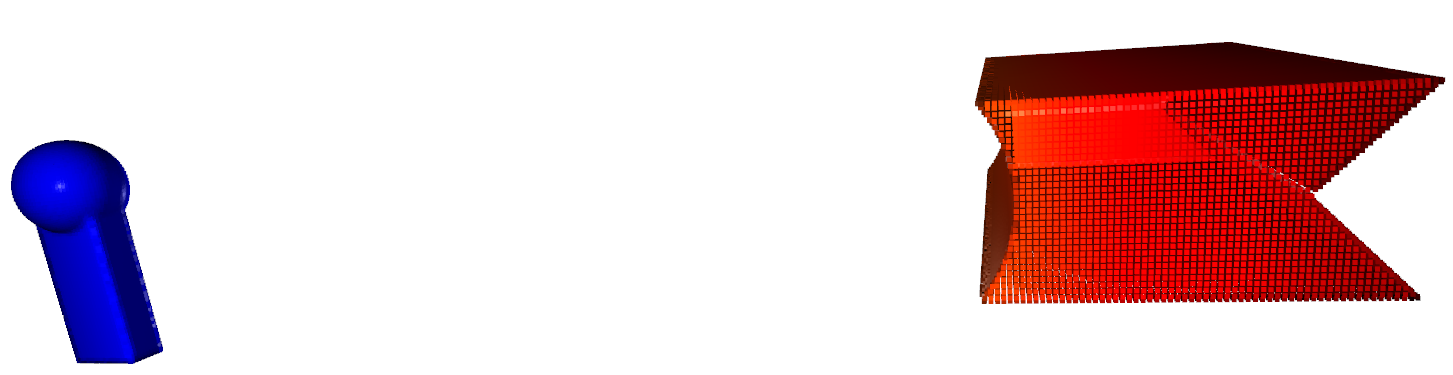
Roughly registered clouds

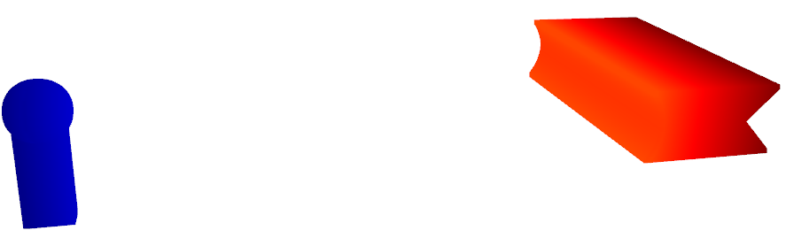
The clouds can finally be fine aligned thanks to ICP :

# Perform ICP
distance_threshold = voxelsize * 0.4
finereg_result = o3d.pipelines.registration.registration_icp(moved_down_pcd, downpcd, distance_threshold)

moved_down_pcd.transform(finereg_result.transformation)
o3d.visualization.draw_geometries([downpcd,moved_down_pcd])

And you are done with the transformation piepline !

Clustering

You can also isolate parts of a cloud thanks to density-based clustering (here, we color each point following their cluster) :

#Cluster different elements by DBSCAN (density based clustering)
print("Clustering cloud")
start_time = time.time()
with o3d.utility.VerbosityContextManager(o3d.utility.VerbosityLevel.Debug) as cm:
        clusters = downpcd.cluster_dbscan(eps=6, min_points=40, print_progress=True)
        labels = np.array(clusters)
        # eps = distance to neighbors in same cluster
        # min_points = minimal points in cluster to be considered as is
elapsed_time = time.time() - start_time
max_label = labels.max()
print(f"Point cloud has {max_label + 1} clusters | Done in {elapsed_time*1000} [ms]")
display(labels)

colors = plt.get_cmap("rainbow")(labels / (max_label if max_label > 0 else 1))
colors[labels < 0] = 0
pcd.colors = o3d.utility.Vector3dVector(colors[:, :3])
o3d.visualization.draw_geometries([pcd])

Clustered parts (each color is a cluster)

Algorithm Open3D 3D-Algorithm