Kernel Density Estimation#

The Kernel Density Estimation (KDE) is a non-parametric way to estimate the probability density function (PDF) of a continuous random variable, as opposed to the probability mass function (PMF) which is used in the context of discrete random variables (random variables that take values on a countable set).

Theory#

The probability density function of a continuous random variable is the probabilities of occurrence of different possible outcomes of that random variable. The shape of that probability density function across the domain for a random variable is referred to as the probability distribution. Common probability distributions have names: uniform, normal, exponential.

One can use an histogram to identify whether the density looks like a common probability distribution or not. If it’s the case, we can use predefined functions to summarize the relashionship between the observations and their probability. In that case the PDF can be controlled with parameters (parametric density estimation). For example the normal distribution has two parameters: the mean and the standard deviation. Given these two parameters we know the PDF.

Sometimes the distribution may not resemble common probability distribution. This is often the case when the data has two peaks (bimodal distribution) or many peaks (multimodal distribution). In this case the parametric density estimation is not feasible. Instead, an algorithm is used to approximate the the probability distribution of the data without a pre-defined distribution, referred to as a non-parametric method.

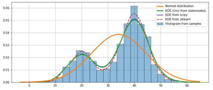
Example of KDE for a bimodal data sample#

import numpy as np
import pandas as pd
import matplotlib.pyplot as plt
import statsmodels.api as sm
from scipy import stats
from scipy.stats.kde import gaussian_kde
from sklearn.neighbors import KernelDensity
from sklearn.model_selection import GridSearchCV

sample1 = np.random.normal(loc=20, scale=5, size=300)
sample2 = np.random.normal(loc=40, scale=5, size=700)
obs_dist = np.hstack((sample1, sample2))

X_plot = np.linspace(obs_dist.min(), obs_dist.max(), 1000)

sm_kde_u = sm.nonparametric.KDEUnivariate(obs_dist)
sm_kde_u.fit()

sp_kde = gaussian_kde(obs_dist)

sk_kde = KernelDensity(kernel='gaussian', bandwidth=1.7).fit(np.array(obs_dist)[:, np.newaxis])
log_dens = sk_kde.score_samples(X_plot[:, np.newaxis])

# ---------------------------------------------------------------------------------------------------

fig = plt.figure(figsize=(12, 5))
ax = fig.add_subplot(111)

# Plot the histrogram
ax.hist(obs_dist, bins=20, density=True, label='Histogram from samples', zorder=5, edgecolor='k', alpha=0.5)

# Plot the true distribution
true_values = (stats.norm.pdf(sm_kde_u.support, obs_dist.mean(), obs_dist.std()))
ax.plot(sm_kde_u.support, true_values, lw=3, label='Normal distribution', zorder=15)

# Plot the KDEs
ax.plot(sm_kde_u.support, sm_kde_u.density, lw=3, label='KDE (Uni) from statsmodels', zorder=10)
ax.plot(X_plot, sp_kde(X_plot), 'b', label="KDE from scipy")
ax.plot(X_plot, np.exp(log_dens), 'r', lw=2, linestyle='--', label="KDE from sklearn")

ax.legend(loc='best')
ax.grid(True, zorder=-5)

We can use the cross-validation method with GridSearchCV from sklearn to find to best bandwidth:

grid = GridSearchCV(KernelDensity(),
                  {'bandwidth': np.linspace(1, 5, 100)},
                  cv=5) # 5-fold cross-validation
grid.fit(np.array(obs_dist)[:, None])
print(grid.best_params_)
# {'bandwidth': 2.0101010101010104}

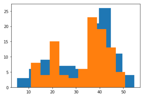
KDEs function from scipy and sklearn have direct method to generate data from the estimated probability:

plt.hist(sp_kde.resample(size=100)[0]);
plt.hist(sk_kde.sample(100));

References#

Machine Learning Python KDE